Simulation of coherent WDM transmission

if 'google.colab' in str(get_ipython()):
    ! git clone -b main https://github.com/edsonportosilva/OptiCommPy
    from os import chdir as cd
    cd('/content/OptiCommPy/')
    ! pip install .

import matplotlib.pyplot as plt
import numpy as np

from optic.dsp.core import pulseShape, firFilter, decimate, symbolSync, pnorm
from optic.models.devices import pdmCoherentReceiver, basicLaserModel

try:
    from optic.models.modelsGPU import manakovSSF
except:
    from optic.models.channels import manakovSSF

from optic.models.tx import simpleWDMTx
from optic.utils import parameters
from optic.dsp.equalization import edc, mimoAdaptEqualizer
from optic.dsp.carrierRecovery import cpr
from optic.comm.metrics import fastBERcalc, monteCarloGMI, monteCarloMI, calcEVM
from optic.plot import pconst, plotPSD

import scipy.constants as const

import logging as logg
logg.basicConfig(level=logg.INFO, format='%(message)s', force=True)
import time

d:\edson\anaconda3\envs\opticommpy-env\Lib\site-packages\cupyx\jit\_interface.py:173: FutureWarning: cupyx.jit.rawkernel is experimental. The interface can change in the future.
  cupy._util.experimental('cupyx.jit.rawkernel')

from IPython.core.display import HTML
from IPython.core.pylabtools import figsize

HTML("""
<style>
.output_png {
    display: table-cell;
    text-align: center;
    vertical-align: middle;
}
</style>
""")

figsize(10, 3)

%load_ext autoreload
%reload_ext autoreload
#%load_ext line_profiler

Summary

OptiCommPy is a Python package for simulating optical communication systems, including Wavelength Division Multiplexing (WDM) systems. This notebook shows an example of how to use OptiCommPy to run a simulation of a coherent WDM system with several modulated co-propagating optical carriers.

Transmitter

The initial step involves defining a comprehensive set of parameters for the WDM transmitters. The table below outlines a specific WDM system configuration where \(11\times32\)GBd PDM-16QAM carriers are generated, following a frequency grid of 37.5 GHz that is centered precisely at the optical frequency of 193.1 THz. Each carrier is modulated with a Nyquist spectrum, by means of a root-raised-cosine (RRC) pulse-shaping filter with a rolloff factor of 0.01. The continuous-wave (CW) lasers utilized in this setup are characterized by linewidths of 100 kHz, with each modulated carrier boasting an output power of -2 dBm.

Parameter	Description	Value
M	Order of the modulation format	16
Rs	Symbol rate [baud]	32e9
SpS	Samples per symbol	16
pulseType	Type of pulse shaping filter	‘rrc’
nFilterTaps	Number of pulse shaping filter coefficients	1024
pulseRollOff	RRC rolloff	0.01
powerPerChannel	Power per WDM channel [dBm]	-2
nChannels	Number of WDM channels	11
Fc	Central frequency of the WDM spectrum [Hz]	193.1e12
laserLinewidth	Laser linewidth [Hz]	100e3
wdmGridSpacing	WDM grid spacing [Hz]	37.5e9
nPolModes	Number of polarization modes	2
nBits	Total number of bits per polarization	400000

The number of samples per symbol (SpS) adopted in the simulation is set to 16, meaning that the signals are represented at a corresponding sampling rate (Fs) of Fs = 16\(\times\)Rs = 512 GSa/s, where Rs is the symbol rate (i.e. 32GBd). The total bandwidth simulated in this setup is 11$:nbsphinx-math:`times`$37.5 GHz = 412.5 GHz, which is below Fs, thus avoiding aliasing in the extremes of the spectrum. The total simulated interval corresponds to 100000 signaling periods, corresponding to 400000 bits transmitted per polarization per WDM carrier.

Polarization multiplexed WDM signal generation

# Transmitter parameters:
paramTx = parameters()
paramTx.M   = 16  # order of the modulation format
paramTx.Rs  = 32e9 # symbol rate [baud]
paramTx.SpS = 16  # samples per symbol
paramTx.pulseType = 'rrc' # pulse shaping filter
paramTx.nFilterTaps = 1024 # number of pulse shaping filter coefficients
paramTx.pulseRollOff = 0.01 # RRC rolloff
paramTx.powerPerChannel = -2 # power per WDM channel [dBm]
paramTx.nChannels = 11 # number of WDM channels
paramTx.Fc = 193.1e12 # central optical frequency of the WDM spectrum
paramTx.laserLinewidth = 100e3 # laser linewidth in Hz
paramTx.wdmGridSpacing = 37.5e9 # WDM grid spacing
paramTx.nPolModes = 2  # number of signal modes [2 for polarization multiplexed signals]
paramTx.nBits = int(np.log2(paramTx.M)*1e5) # total number of bits per polarization
paramTx.seed = 123 # random seed for bit generation

# generate WDM signal
sigWDM_Tx, symbTx_, paramTx = simpleWDMTx(paramTx)

channel 0        fc : 192.9125 THz
  mode #0        power: -5.01 dBm
  mode #1        power: -5.01 dBm
channel 0        power: -2.00 dBm

channel 1        fc : 192.9500 THz
  mode #0        power: -5.01 dBm
  mode #1        power: -5.01 dBm
channel 1        power: -2.00 dBm

channel 2        fc : 192.9875 THz
  mode #0        power: -5.01 dBm
  mode #1        power: -5.01 dBm
channel 2        power: -2.00 dBm

channel 3        fc : 193.0250 THz
  mode #0        power: -5.01 dBm
  mode #1        power: -5.01 dBm
channel 3        power: -2.00 dBm

channel 4        fc : 193.0625 THz
  mode #0        power: -5.01 dBm
  mode #1        power: -5.01 dBm
channel 4        power: -2.00 dBm

channel 5        fc : 193.1000 THz
  mode #0        power: -5.01 dBm
  mode #1        power: -5.01 dBm
channel 5        power: -2.00 dBm

channel 6        fc : 193.1375 THz
  mode #0        power: -5.01 dBm
  mode #1        power: -5.01 dBm
channel 6        power: -2.00 dBm

channel 7        fc : 193.1750 THz
  mode #0        power: -5.01 dBm
  mode #1        power: -5.01 dBm
channel 7        power: -2.00 dBm

channel 8        fc : 193.2125 THz
  mode #0        power: -5.01 dBm
  mode #1        power: -5.01 dBm
channel 8        power: -2.00 dBm

channel 9        fc : 193.2500 THz
  mode #0        power: -5.01 dBm
  mode #1        power: -5.01 dBm
channel 9        power: -2.00 dBm

channel 10       fc : 193.2875 THz
  mode #0        power: -5.01 dBm
  mode #1        power: -5.01 dBm
channel 10       power: -2.00 dBm

total WDM signal power: 8.41 dBm

Nonlinear fiber model

Vector Manakov Equation

When considering two polarizations propagating over an optical fiber, the Manakov model can be used to describe the coupled propagation of two orthogonal polarization components, taking into account their mutual interactions and the characteristics of the fiber such as attenuation, nonlinearity and dispersion.

The vectorial Manakov equation is a system of coupled nonlinear Schrödinger equations (NLSEs) for the two polarizations, \(x\) and \(y\), written in the following form:

\[\frac{\partial E_x(z,t)}{\partial z} +\frac{\alpha}{2}E_x(z,t) + j\frac{\beta_2}{2}\frac{\partial^2 E_x(z,t)}{\partial t^2} - j\frac{8\gamma}{9}\left(|E_x(z,t)|^2 + |E_y(z,t)|^2\right)E_x(z,t) = 0\]

\[\frac{\partial E_y(z,t)}{\partial z} +\frac{\alpha}{2}E_y(z,t) + j\frac{\beta_2}{2}\frac{\partial^2 E_y(z,t)}{\partial t^2} - j\frac{8\gamma}{9}\left(|E_x(z,t)|^2 + |E_y(z,t)|^2\right)E_y(z,t) = 0\]

where:

• \(E_x(z,t)\) and \(E_y(z,t)\) are the complex-valued electric field envelopes for the \(x\) and \(y\) polarizations, respectively.

• \(z\) is the propagation distance along the fiber.

• \(t\) is time.

• \(\beta_2\) is the group velocity dispersion (GVD) parameter of the fiber.

• \(\gamma\) is the nonlinear coefficient of the fiber.

These equations model the linear effects of fiber attenuation and chromatic dispersion, and the nonlinear distortions originated from self-phase modulation (SPM), cross-phase modulation (XPM) and four-wave-mixing (FWM). The Manakov model is formulated under the assumption that the impact of polarization mode dispersion (PMD) effects is significantly smaller compared to the nonlinear effects and the characteristic length scales involved. This assumption implies that the beat length associated with PMD is much shorter than the nonlinear effective length of the fiber. In this context, the resulting nonlinear term in the Manakov equation represents an averaged effect of the fiber’s nonlinearity, accounting for the rapid variations in the polarization states as the optical signal propagates through the fiber. This averaging captures the overall influence of the fiber’s nonlinearity on the signal, considering the dynamic changes in polarization states over short distances.

Nonlinear fiber propagation with a symmetric split-step Fourier method

The Split-Step Fourier Method (SSFM) is a powerful numerical technique extensively utilized in optical fiber communications to solve the NLSE, which governs the propagation of optical signals in fibers. It’s designed to handle the intricate interplay of linear and nonlinear effects accumulated over long propagation distances. The fundamental concept of SSFM involves breaking down the complicated task of describing the signal propagation over long distances of fiber into a iterative sequence of simple calculation steps, involving time and frequency domain representations of the propagating signal. By assuming the independence of linear and nonlinear effects at each small propagation step, they can be applied to the signals independently in an iterative manner, ensuring accurate modeling of optical phenomena.

The coupled Manakov equations described above can be numerically integrated via split-step Fourier methods. A pseudocode for the SSFM algorithm is shown below.

Pseudocode of the SSFM that solves the Manakov propagation model

1. Initialize:

   • Parameters: \(L\), \(h_z\), \(\Delta t\), \(E_x(z=0,t)\), \(E_x(z=0,t)\) (input fields)

2. Loop for propagation over :math:`L`:

   for \(z = 0\) to \(L\) with step \(h_z\):

   Half-linear step:

   • \(E_x(z,t)\gets \mathrm{IFFT}\left\lbrace\exp\left[\left(-\frac{\alpha}{2}-j\frac{\beta_2 \omega^2}{2}\right) h_z/2\right] \mathrm{FFT}[E_x(z,t)]\right\rbrace\)

   • \(E_y(z,t)\gets \mathrm{IFFT}\left\lbrace\exp\left[\left(-\frac{\alpha}{2}-j\frac{\beta_2 \omega^2}{2}\right) h_z/2\right] \mathrm{FFT}[E_y(z,t)]\right\rbrace\)

   Nonlinear phase rotation step:

   • \(E_x(z,t) \gets E_x(z,t)\exp\left[-j8\gamma/9 \left(|E_x(z,t)|^2 + |E_y(z,t)|^2\right) h_z\right]\)

   • \(E_y(z,t) \gets E_y(z,t)\exp\left[-j8\gamma/9 \left(|E_x(z,t)|^2 + |E_y(z,t)|^2\right) h_z\right]\)

   Half-linear step:

   • \(E_x(z,t)\gets \mathrm{IFFT}\left\lbrace\exp\left[\left(-\frac{\alpha}{2}-j\frac{\beta_2 \omega^2}{2}\right) h_z/2\right] \mathrm{FFT}[E_x(z,t)]\right\rbrace\)

   • \(E_y(z,t)\gets \mathrm{IFFT}\left\lbrace\exp\left[\left(-\frac{\alpha}{2}-j\frac{\beta_2 \omega^2}{2}\right) h_z/2\right] \mathrm{FFT}[E_y(z,t)]\right\rbrace\)

   Propagation: $ z = z + h_z$

3. Output: Final \(E_x(z=L,t)\), \(E_y(z=L,t)\) for analysis.

Parameter	Description	Value
Ltotal	Total link distance [km]	700
Lspan	Span length [km]	50
alpha	Fiber loss parameter [dB/km]	0.2
D	Fiber dispersion parameter [ps/nm/km]	16
gamma	Fiber nonlinear parameter [1/(W.km)]	1.3
Fc	Central optical frequency of the WDM spectrum	193.1e12
hz	Step-size of the split-step Fourier method [km]	0.5
maxIter	Maximum number of convergence iterations per step	5
tol	Error tolerance per step	1e-5
nlprMethod	Use adaptive step-size based on maximum nonlinear phase-shift	True
maxNlinPhaseRot	Maximum nonlinear phase-shift per step	2e-2
prgsBar	Show progress bar	True
Fs	Sampling rate	Calculated

# optical channel parameters
paramCh = parameters()
paramCh.Ltotal = 700     # total link distance [km]
paramCh.Lspan  = 50      # span length [km]
paramCh.alpha = 0.2      # fiber loss parameter [dB/km]
paramCh.D = 16           # fiber dispersion parameter [ps/nm/km]
paramCh.gamma = 1.3      # fiber nonlinear parameter [1/(W.km)]
paramCh.Fc = paramTx.Fc  # central optical frequency of the WDM spectrum
paramCh.hz = 0.5         # step-size of the split-step Fourier method [km]
paramCh.maxIter = 5      # maximum number of convergence iterations per step
paramCh.tol = 1e-5       # error tolerance per step
paramCh.nlprMethod = True # use adaptive step-size based o maximum nonlinear phase-shift
paramCh.maxNlinPhaseRot = 2e-2 # maximum nonlinear phase-shift per step
paramCh.prgsBar = True   # show progress bar
paramCh.Fs = paramTx.Rs*paramTx.SpS # sampling rate
paramCh.seed = 456 # random seed for noise generation

# nonlinear signal propagation
sigWDM = manakovSSF(sigWDM_Tx, paramCh)

Running Manakov SSF model on GPU...

Optical WDM spectrum before and after transmission

# plot psd
Fs = paramCh.Fs
fig,_ = plotPSD(sigWDM_Tx, Fs, paramTx.Fc, label='Tx');
fig, ax = plotPSD(sigWDM, Fs, paramTx.Fc, fig=fig, label='Rx');
fig.set_figheight(3)
fig.set_figwidth(10)
ax.set_title('optical WDM spectrum');

Coherent detection, digital signal processing and data demodulation

Optical coherent receiver frontend

# Receiver

# parameters
chIndex  = int(np.floor(paramTx.nChannels/2))      # index of the channel to be demodulated
freqGrid = paramTx.wdmFreqGrid
symbTx = symbTx_[:,:,chIndex]

print('Demodulating channel #%d , fc: %.4f THz, λ: %.4f nm\n'\
      %(chIndex, (paramCh.Fc + freqGrid[chIndex])/1e12, const.c/(paramCh.Fc + freqGrid[chIndex])/1e-9))


# local oscillator (LO) parameters:
FO  = -128e6                 # frequency offset
paramLO = parameters()
paramLO.P = 10              # power in dBm
paramLO.lw = 100e3          # laser linewidth
paramLO.RIN_var = 0
paramLO.Ns = len(sigWDM)
paramLO.Fs = Fs
paramLO.seed = 789 # random seed for noise generation
paramLO.freqShift = freqGrid[chIndex] + FO  # downshift of the channel to be demodulated add frequency offset

# generate CW laser LO field
sigLO = basicLaserModel(paramLO)

print('Local oscillator P: %.2f dBm, lw: %.2f kHz, FO: %.2f MHz\n'\
      %(paramLO.P, paramLO.lw/1e3, FO/1e6))

# polarization multiplexed coherent optical receiver

# Frontend parameters
paramFE = parameters()
paramFE.Fs = Fs
paramFE.polRotation = np.pi/3    # input polarization rotation angle
paramFE.pdl = 0                  # Polarization dependent loss
paramFE.polDelay = 4e-12         # Polarization delay
paramFE.phaseImbX = 0*np.pi/180  # IQ phase imbalance polarization X in radians
paramFE.phaseImbY = 0*np.pi/180  # IQ phase imbalance polarization Y in radians
paramFE.ampImbX = 0              # IQ amplitude imbalance polarization X in dB
paramFE.ampImbY = 0              # IQ amplitude imbalance polarization Y in dB

# photodiodes parameters
paramPD = parameters()
paramPD.B = paramTx.Rs
paramPD.Fs = Fs
paramPD.ideal = True
paramPD.seed = 1011

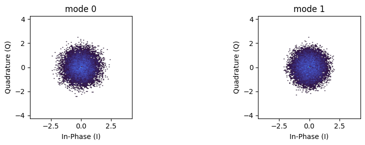
sigRx = pdmCoherentReceiver(sigWDM, sigLO, paramFE, paramPD)

# plot received constellations
pconst(sigRx[0::paramTx.SpS,:], R=3);

Demodulating channel #5 , fc: 193.1000 THz, λ: 1552.5244 nm

Local oscillator P: 10.00 dBm, lw: 100.00 kHz, FO: -128.00 MHz

Matched filtering

# Rx filtering

# Matched filtering
paramPS = parameters()
paramPS.SpS = paramTx.SpS
paramPS.nFilterTaps = paramTx.nFilterTaps
paramPS.rollOff = paramTx.pulseRollOff
paramPS.pulseType = paramTx.pulseType
pulse = pulseShape(paramPS)

start = time.time()
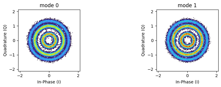
sigRx = firFilter(pulse, sigRx)
end = time.time()
timeMF = end - start
print(f"Matched filtering took {timeMF:.2f} seconds.")

# plot constellations after matched filtering
pconst(sigRx[0::paramTx.SpS,:], R=3);

Matched filtering took 0.40 seconds.

Downsampling to 2 samples/symbol and CD compensation

# decimation
paramDec = parameters()
paramDec.SpSin  = paramTx.SpS
paramDec.SpSout = 2

start = time.time()
sigRx = decimate(sigRx, paramDec)
end = time.time()
timeDec = end - start
print(f"Decimation took {timeDec:.2f} seconds.")

Decimation took 0.12 seconds.

# CD compensation
paramEDC = parameters()
paramEDC.L = paramCh.Ltotal
paramEDC.D = paramCh.D
paramEDC.Fc = paramCh.Fc
paramEDC.Rs = paramTx.Rs
paramEDC.Fs = 2*paramTx.Rs

start = time.time()
sigRx = edc(sigRx, paramEDC)
end = time.time()
timeCDcomp = end - start
print(f"CD compensation took {timeCDcomp:.2f} seconds.")

# plot constellations after CD compensation
pconst(sigRx[0::paramTx.SpS,:], R=3);

# re-synchronization with transmitted sequences
symbRx = symbolSync(sigRx, symbTx, 2)

Running CD compensation...
CD filter length: 392 taps, FFT size: 512

CD compensation took 0.16 seconds.

Power normalization

x = pnorm(sigRx)
d = pnorm(symbRx)

Adaptive equalization

# adaptive equalization parameters
paramEq = parameters()
paramEq.nTaps = 35
paramEq.SpS = paramDec.SpSout
paramEq.numIter = 2
paramEq.storeCoeff = False
paramEq.M = paramTx.M
paramEq.shapingFactor = paramTx.shapingFactor
paramEq.L = [int(0.2*d.shape[0]), int(0.8*d.shape[0])]
paramEq.prgsBar = False

if paramTx.M == 4:
    paramEq.alg = ['cma','cma'] # QPSK
    paramEq.mu = [5e-3, 1e-3]
else:
    paramEq.alg = ['da-rde','rde'] # M-QAM
    paramEq.mu = [5e-3, 5e-4]

start = time.time()
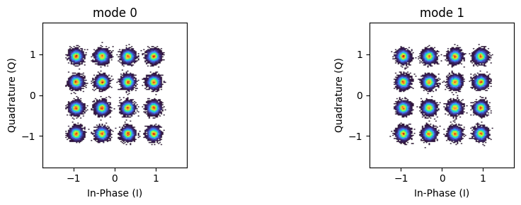
y_EQ = mimoAdaptEqualizer(x, paramEq, d)
end = time.time()
timeEq = end - start
print(f"Adaptive equalization took {timeEq:.2f} seconds.")

#plot constellations after adaptive equalization
discard = 5000
pconst(y_EQ[discard:-discard,:], R=1.5);

Running adaptive equalizer...
da-rde - training stage #0
da-rde pre-convergence training iteration #0
da-rde MSE = 0.033816.
da-rde pre-convergence training iteration #1
da-rde MSE = 0.027277.
rde - training stage #1
rde MSE = 0.015509.

Adaptive equalization took 0.69 seconds.

Carrier frequency offset and phase recovery

paramCPR = parameters()
paramCPR.alg = 'bps'
paramCPR.M   = paramTx.M
paramCPR.constType = paramTx.constType
paramCPR.shapingFactor = paramTx.shapingFactor
paramCPR.N   = 25
paramCPR.B   = 64
paramCPR.returnPhases = False
paramCPR.Ts = 1/paramTx.Rs

start = time.time()
y_CPR = cpr(y_EQ, paramCPR)
end = time.time()
timeCPR = end - start
print(f"CPR took {timeCPR:.2f} seconds.")

discard = 5000

#plot constellations after CPR
pconst(y_CPR[discard:-discard,:]);

Running frequency offset compensation...
Estimated frequency offset (MHz): [128.24 128.24]
Running BPS carrier phase recovery...
Estimated linewidth: 376.087 kHz

CPR took 5.21 seconds.

Evaluate transmission metrics

ind = np.arange(discard, d.shape[0]-discard)

# remove phase and polarization ambiguities for QPSK signals
if paramTx.M == 4:
    d = symbTx
    # find rotations after CPR and/or polarizations swaps possibly added at the output the adaptive equalizer:
    rot0 = [np.mean(pnorm(symbTx[ind,0])/pnorm(y_CPR[ind,0])), np.mean(pnorm(symbTx[ind,1])/pnorm(y_CPR[ind,0]))]
    rot1 = [np.mean(pnorm(symbTx[ind,1])/pnorm(y_CPR[ind,1])), np.mean(pnorm(symbTx[ind,0])/pnorm(y_CPR[ind,1]))]

    if np.argmax(np.abs(rot0)) == 1 and np.argmax(np.abs(rot1)) == 1:
        y_CPR_ = y_CPR.copy()
        # undo swap and rotation
        y_CPR[:,0] = pnorm(rot1[np.argmax(np.abs(rot1))]*y_CPR_[:,1])
        y_CPR[:,1] = pnorm(rot0[np.argmax(np.abs(rot0))]*y_CPR_[:,0])
    else:
        # undo rotation
        y_CPR[:,0] = pnorm(rot0[np.argmax(np.abs(rot0))]*y_CPR[:,0])
        y_CPR[:,1] = pnorm(rot1[np.argmax(np.abs(rot1))]*y_CPR[:,1])


BER, SER, SNR = fastBERcalc(y_CPR[ind,:], d[ind,:], paramTx.M, 'qam',px=paramTx.pmf)
GMI, NGMI = monteCarloGMI(y_CPR[ind,:], d[ind,:], paramTx.M, 'qam',px=paramTx.pmf)
MI       = monteCarloMI(y_CPR[ind,:], d[ind,:], paramTx.M, 'qam',px=paramTx.pmf)
EVM      = calcEVM(y_CPR[ind,:], paramTx.M, 'qam', d[ind,:])

print('      pol.X      pol.Y      ')
print(' SER: %.2e,  %.2e'%(SER[0], SER[1]))
print(' BER: %.2e,  %.2e'%(BER[0], BER[1]))
print(' SNR: %.2f dB,  %.2f dB'%(SNR[0], SNR[1]))
print(' EVM: %.2f %%,    %.2f %%'%(EVM[0]*100, EVM[1]*100))
print('  MI: %.2f bits, %.2f bits'%(MI[0], MI[1]))
print(' GMI: %.2f bits, %.2f bits'%(GMI[0], GMI[1]))
print('NGMI: %.2f,      %.2f'%(NGMI[0], NGMI[1]))

      pol.X      pol.Y
 SER: 2.22e-05,  1.11e-04
 BER: 5.56e-06,  2.78e-05
 SNR: 20.69 dB,  20.66 dB
 EVM: 0.86 %,    0.86 %
  MI: 4.00 bits, 4.00 bits
 GMI: 4.00 bits, 4.00 bits
NGMI: 1.00,      1.00

Summary of processing time required by each DSP block

print(f"{'-'*42}")
print(f"| {'DSP execution time benchmark':<30} | {'Time':<5} |")
print(f"| {'-'*30} | {'-'*5} |")
print(f"| {'Matched filtering':<30} | {timeMF:.2f} s|")
print(f"| {'CD compensation':<30} | {timeCDcomp:.2f} s|")
print(f"| {'Decimation':<30} | {timeDec:.2f} s|")
print(f"| {'Adaptive equalization':<30} | {timeEq:.2f} s|")
print(f"| {'Carrier phase recovery':<30} | {timeCPR:.2f} s|")
print(f"{'-'*42}")
print(f"| {'Total':<30} | {timeMF + timeCDcomp + timeDec + timeEq + timeCPR:.2f} s|")
print(f"{'-'*42}")

------------------------------------------
| DSP execution time benchmark   | Time  |
| ------------------------------ | ----- |
| Matched filtering              | 0.40 s|
| CD compensation                | 0.16 s|
| Decimation                     | 0.12 s|
| Adaptive equalization          | 0.69 s|
| Carrier phase recovery         | 5.21 s|
------------------------------------------
| Total                          | 6.58 s|
------------------------------------------

References

[1] D. Marcuse, C. R. Menyuk, e P. K. A. Wai, “Application of the Manakov-PMD equation to studies of signal propagation in optical fibers with randomly varying birefringence”, Journal of Lightwave Technology, vol. 15, nº 9, p. 1735–1745, 1997, doi: 10.1109/50.622902.

[2] S. J. Savory, “Digital coherent optical receivers: Algorithms and subsystems”, IEEE Journal on Selected Topics in Quantum Electronics, vol. 16, nº 5, p. 1164–1179, set. 2010, doi: 10.1109/JSTQE.2010.2044751.

[3] K. Kikuchi, “Fundamentals of Coherent Optical Fiber Communications”, J. Lightwave Technol., JLT, vol. 34, nº 1, p. 157–179, jan. 2016.